M/M/1 Queues : Exercises

Introduction

The problems below all involve a continuous time Markov chains that can be used to model the behavior of queues. Such Markov chains have a stationary distribution when the time between arrivals is greater than the average service time. Further notice how this model for queues can appear in a range of different guises.

Example problems

Click on the problems to reveal the solution

Problem 1

First of all notice that the number of books in this shop is a Markov chain in continuous time because the number of books at the next instant in time depends only on the current number of books and because books arrive at random times. This is not a particularly sensible model as you are assumign that the rate that books and donated and bought is time indepdnent. This assumption is obviously not valid if the shop is busier on weekends. However, the question tells us to use this model so lets continus. Further note that the question tells us nothing about any limit on the number of books that can be held in the shop so we should assume that the continuous time Markov chain that we are going to use to model the number of books in the shop at any given time has an infinite number of states. In other words, the transition graph for this problem is going to look like this:


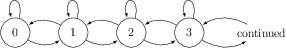
In addition the jump rate matrix is going to have an infinite number of rows and columns as shown below: $$ \mathbf{Q} = \left( \begin{matrix} -\lambda & \lambda & 0 & 0 & 0 & \dots & 0 & 0 \\ \mu & -\lambda-\mu & \lambda & 0 & 0 & \dots & 0 & 0 \\ 0 & \mu & -\lambda-\mu & \lambda & 0 & \dots & 0 & 0 \\ \vdots & \vdots & \vdots & \vdots & \vdots & \ddots & \vdots & \vdots \\ \end{matrix} \right) $$ Finding the stationary distribution is straightforward. To do so we need to find some non trivial $\pi$ that satisfies: $$ \pi \mathbf{Q} = 0 $$ In other words we are trying to find the row vector $\pi$ that satisfies the matrix equation below: $$ \left( \begin{matrix} \pi_0 & \pi_1 & \pi_2 \dots & \pi_N \end{matrix} \right) \left( \begin{matrix} -\lambda & \lambda & 0 & 0 & 0 & \dots & 0 & 0 \\ \mu & -\lambda-\mu & \lambda & 0 & 0 & \dots & 0 & 0 \\ 0 & \mu & -\lambda-\mu & \lambda & 0 & \dots & 0 & 0 \\ \vdots & \vdots & \vdots & \vdots & \vdots & \ddots & \vdots & \vdots \\ \end{matrix} \right) = 0 $$ When this system of equations is multiplied out we find that: $$ \pi_0 = \frac{\mu}{\lambda} \pi_1 \qquad \mu \pi_2 = (\lambda + \mu ) \pi_1 - \lambda \pi_0 = ( \lambda + \mu ) \pi_1 - \mu \pi_1 = \lambda \pi_1 \qquad \rightarrow \qquad \pi_2 = \frac{\lambda}{\mu}\pi_1 $$ The equations above follow the simple pattern shown below: $$ \pi_{n+1} = \frac{\lambda}{\mu} \pi_{n-1} $$ We can thus solve this family of equations recursively and get to: $$ \pi_{n} = \left(\frac{\lambda}{\mu} \right)^n \pi_0 $$ We now use normalization to determine $\pi_0$ $$ 1 = \sum_{n=0}^\infty \left(\frac{\lambda}{\mu} \right)^n \pi_0 \qquad \rightarrow \qquad \pi_0 = 1 - \left(\frac{\lambda}{\mu}\right) $$ Notice that in this step we have used a well known result on the sum of the geometric series: $\sum_{k=0}^\infty a^k = \frac{1}{1-a}$.

In closing note that the question asks for the expected number of books in the shop. Given we have the result above for the stationary distribution this expectation is clearly: \[ \mathbb{E}(X) = \sum_{i=0}^\infty i \pi_i = \sum_{i=0}^\infty i \left(1 - \frac{\lambda}{\mu}\right)\left(\frac{\lambda}{\mu}\right)^i = \left(1 - \frac{\lambda}{\mu}\right) \sum_{i=0}^\infty i \left(\frac{\lambda}{\mu}\right)^i = \frac{ \frac{\lambda}{\mu} }{1-\frac{\lambda}{\mu}} \] The result asked for in the question is obtained by multiplying top and bottom by $\mu$.

Problem 2

First of all notice that the amount of energy in the batteries is a Markov chain in continuous time because the energy at the next instant in time depends only on the current level of energy in the battery. Furthermore, the addition of energy and the removal of energy is a continuous time random process and as a result the model that emerges will be a continuous time Markov chain. Notice, however, that the batteries have a finite capacity. This is important as it means that there is a difference between the model that is the solution of this problem and the model that is the solution to the problem in the previous question. This difference can be seen when you compare the transition graphs for this problem, which is shown below:


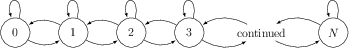
and the transition graph in the previous problem. The number of states in the transition graph for this problem is finite, whereas the number of states in the previous problem was infinite. The fact that we have only a finite number of states in this case also introduces differences in the jump rate matrix as shown below: $$ \mathbf{Q} = \left( \begin{matrix} -\lambda & \lambda & 0 & 0 & 0 & \dots & 0 & 0 \\ \mu & -\lambda-\mu & \lambda & 0 & 0 & \dots & 0 & 0 \\ 0 & \mu & -\lambda-\mu & \lambda & 0 & \dots & 0 & 0 \\ \vdots & \vdots & \vdots & \vdots & \vdots & \ddots & \vdots & \vdots \\ 0 & 0 & 0 & 0 & 0 & \dots & \mu & -\mu \end{matrix} \right) $$ This jump rate matrix for this problem is an $n \times n$ matrix, whereas the jump rate matrix in the previous question had an infinite number of rows and an infinite number of columns.

Having focussed on the differences the process of finding the stationary distribution is relatively similar. As in question one we are looking for some non trivial $\pi$ that satisfies: $$ \pi \mathbf{Q} = 0 $$ In other words we are trying to find the row vector $\pi$ that satisfies the matrix equation below: $$ \left( \begin{matrix} \pi_0 & \pi_1 & \pi_2 \dots & \pi_N \end{matrix} \right) \left( \begin{matrix} -\lambda & \lambda & 0 & 0 & 0 & \dots & 0 & 0 \\ \mu & -\lambda-\mu & \lambda & 0 & 0 & \dots & 0 & 0 \\ 0 & \mu & -\lambda-\mu & \lambda & 0 & \dots & 0 & 0 \\ \vdots & \vdots & \vdots & \vdots & \vdots & \ddots & \vdots & \vdots \\ 0 & 0 & 0 & 0 & 0 & \dots & \mu & -\mu \end{matrix} \right) = 0 $$ When this system of equations is multiplied out we find that: $$ \pi_0 = \frac{\mu}{\lambda} \pi_1 \qquad \lambda \pi_2 = (\lambda + \mu ) \pi_1 - \lambda \pi_0 = ( \lambda + \mu ) \pi_1 - \mu \pi_1 = \mu \pi_1 \qquad \rightarrow \qquad \pi_2 = \frac{\lambda}{\mu}\pi_1 $$ The equations above follow the simple pattern shown below: $$ \pi_{n+1} = \frac{\lambda}{\mu} \pi_{n-1} $$ We can thus solve this family of equations recursively and get to: $$ \pi_{n} = \left(\frac{\lambda}{\mu} \right)^n \pi_0 $$ We then use the normalization condition to determine $\pi_0$ $$ 1 = \sum_{n=0}^C\left(\frac{\lambda}{\mu} \right)^n \pi_0 \qquad \rightarrow \qquad \pi_0 = \frac{ 1 - \frac{\lambda}{\mu} }{1 - \left(\frac{\lambda}{\mu}\right)^{C+1} } $$ Notice that in this step there is again a difference between what is done here and what was done for a queue that does not have finite capacity. Obviously, if we only only have $(C+1)$ states $\pi$ has only $(C+1)$ elements and thus the sum above has a finite number of terms. We thus have to replace the result on the geometric series that we used in the previous case with the equally well-known result for the sum of the first $(C+1)$ terms in the gemetric series $\sum_{k=0}^C a^k = \frac{1 - a^{C+1}}{1-a}$.

In closing note that the questions asks for the expected level of energy in the batteries. Given we have the result above for the stationary distribution this expectation is clearly: $$ \mathbb{E}(X) = \sum_{n=0}^C n \pi_n = \frac{ 1 - \frac{\lambda}{\mu} }{ 1 - \left( \frac{\lambda}{\mu} \right)^{C+1}} \sum_{n=0}^C n \left( \frac{\lambda}{\mu} \right)^n $$

Problem 3

In this question we have multiple servers. Clearly, this is only going to affect the rate at which people are served. The fact that there are multiple servers is not going to affect the rate at which customers arrive so we thus know that all the $k(k+1)$ of our Jump rate matrix, $\mathbf{Q}$, will remain equal to $\lambda$ just as they have been in the previous questions. Further note that customers still arrive one at at time so all the $k(k+n)$ where $n>1$ elements of $\mathbf{Q}$ will still be equal to zero. Furthermore, although there are multiple servers, we will still assume that it is impossible for two customers to get out of the service system at exacly the same instant in time. As such all the $k(k-n)$ where $n>1$ elements of $\mathbf{Q}$ will also still be zero. In other words, the fact that there are multiple servers will only affect the $k(k-1)$ elements of $\mathbf{Q}$ and by extension the $kk$ elements of $\mathbf{Q}$. To find the values of the $k(k-1)$ elements of $\mathbf{Q}$ we need to remember that in the M/M/1 queue we assume that the time a customer spends being served is given by an exponentially distributed random variable. If we thus have $j$ people being served at once the time taken for the number of people in the queue (which remember counts the number of people standing in the queue and the number of people being served) will be the minimum of $k$ identically-distributed, independent, exponential random variables. That is to say the time taken, $T$, for the length of the queue to decrease by one is given by: $$ T = \min( X_1, X_2, \dots , X_j ) $$ where all the $X_i$ here are exponentially distributed random variables with cumulative probability distributions equal to: $$ F_X(x) = 1 - e^{-\mu x} $$ We can find a cumulative probability distribution function for $T$ and hence the rate parameter that will enter our Jump rate matrix by noting that: $$ P(T>t) = P( X_1>t \wedge X_2>t \wedge \dots \wedge X_j>t ) = P(X_1>t) P(X_2>t) \dots P(X_j>t) = \prod_{i=1}^j P(X_i>t) $$ Notice the second equality here holds because $X_1,X_2,\dots,X_j$ are all independent random variables. We next remember that $P(X_i>t)=e^{-\mu x}$, which brings us to: $$ P(T>t) = \prod_{i=1}^j P(X_i>t) = \prod_{i=1}^j e^{-\mu t} = \left( e^{-\mu t} \right)^j = e^{-j \mu t} $$ We thus find that if one person is being served the rate at which the queues length will decrease by one is equal to $\mu$. If two people are being served then the rate at which the queues length will decrease by one is equal to $2\mu$. If $s$ people are being served then the rate at which the queues length will decrease by one is given by $s\mu$. When all this information is inserted into the jump rate matrix we find: $$ \mathbf{Q} = \left( \begin{matrix} -\lambda & \lambda & 0 & 0 & \dots & 0 & 0 & 0 & 0 & 0 & \dots \\ \mu & -\lambda-\mu & \lambda & 0 & \dots & 0 & 0 & 0 & 0 & 0 & \dots \\ 0 & 2\mu & -\lambda-2\mu & \lambda & \dots & 0 & 0 & 0 & 0 & 0 & \dots \\ \vdots & \vdots & \vdots & \vdots & \ddots & \vdots & \vdots & \vdots & \vdots & \vdots & \dots \\ 0 & 0 & 0 & 0 & \dots & (s-1)\mu & -\lambda - (s-1)\mu & \lambda & 0 & 0 & \dots \\ 0 & 0 & 0 & 0 & \dots & 0 & s\mu & -\lambda - s\mu & \lambda & 0 & \dots \\ 0 & 0 & 0 & 0 & \dots & 0 & 0 & s\mu & -\lambda - s\mu & \lambda & \dots \\ \vdots & \vdots & \vdots & \vdots & \vdots & \vdots & \vdots & \vdots & \vdots & \vdots & \ddots \end{matrix} \right) $$ The question tells us to find the elements of the stationary distribution by using the detailed balance condition. It is worth noting at this stage that we could have used the same approach in questions 1 and 2. Remember the detailed balance condition tells us: $$ \pi_i Q_{ij} = \pi_j Q_{ji} $$ So for this problem we can find equations such as the following directly by using the detailed balance condition and the matrix above: $$ \pi_0 \lambda = \pi_1 \mu \qquad \textrm{and} \qquad \pi_1 \lambda =\pi_2 2\mu \qquad \textrm{and} \qquad \pi_{s-1} \lambda =\pi_s s\mu \qquad \textrm{and} \qquad \pi_{s} \lambda =\pi_{s+1} s\mu $$ In fact if we look at these results we notce the following pattern for those involving the small elements of $\pi$ i.e. those $\pi_n$ values with $n \le s$: $$ n \mu \pi_n = \lambda \pi_{n-1} \qquad \rightarrow \qquad \pi_n = \left(\frac{\lambda}{ n \mu} \right) \pi_{n-1} \qquad \textrm{for} \quad n \le s $$ Meanwhile, for those elements with $n>s$ we find that: $$ s \mu \pi_n = \lambda \pi_{n-1} \qquad \rightarrow \qquad \pi_n = \left(\frac{\lambda}{ s \mu} \right) \pi_{n-1} \qquad \textrm{for} \quad n > s $$ If we solve the first of these sets of equtions recursively we find: $$ \begin{aligned} \pi_1 & = \left(\frac{\lambda}{1 \mu} \right) \pi_0 \\ \pi_2 & = \left(\frac{\lambda}{2 \mu} \right) \pi_1 \qquad \rightarrow \qquad \pi_2 = \frac{1}{2!} \left(\frac{\lambda}{\mu} \right)^2 \pi_0 \\ \pi_3 & = \left(\frac{\lambda}{3 \mu} \right) \pi_3 \qquad \rightarrow \qquad \pi_2 = \frac{1}{3!} \left(\frac{\lambda}{\mu} \right)^3 \pi_0 \end{aligned} $$ The general rule shown below thus emerges for all the elements of $\pi$ with $n \le s$: $$ \pi_n = \frac{1}{n!} \left(\frac{\lambda}{\mu} \right)^n \pi_0 $$ If we now focus on the second general rule for $n>s$. We have: $$ \begin{aligned} \pi_{s+1} & = \left(\frac{\lambda}{ s \mu} \right)^2 \pi_{s-1} \\ \pi_{s+2} & = \left(\frac{\lambda}{ s \mu} \right)^3 \pi_{s-1} \\ \pi_{s+3} & = \left(\frac{\lambda}{ s \mu} \right)^4 \pi_{s-1} \end{aligned} $$ These solutions all clearly follow the template that we were asked to show in the question; namely: $ \pi_n = \left(\frac{\lambda}{ s \mu} \right)^{n-s+1} \pi_{s-1} $

Contact Details

School of Mathematics and Physics,
Queen's University Belfast,
Belfast,
BT7 1NN

Email: g.tribello@qub.ac.uk
Website: mywebsite