Markov chains in continuous times : Exercises

Introduction

The problems below all involve models that are constructed using the theory of Markov chains in continuous time. One of the central results in this theory is the Kolmogorov equation: $$ \frac{\textrm{d}P(t)}{\textrm{d}t} = \mathbf{P}(t) \mathbf{Q} $$

Example problems

Click on the problems to reveal the solution

Problem 1

Glaucoma is a disease of the eyes that usually occurs in old aged patients. Its progression, in the absence of treatment, can be modelled as a continuous time Markov chain with three states $X=1$ (mild), $X=2$ (severe) and $X=3$ (near blindness). Direct progression from state $X=1$ to $X=3$ is never observed. However, patients transition from state $X=1$ to $X=2$ with a rate $\lambda_1$ and from state $X=2$ to state $X=3$ with a rate $\lambda_2$. Draw a transition graph that illustrates the progression of the disease and write out the jump rate matrix, $\mathbf{Q}$. Use the jump rate matrix to derive the Kolmogorov forward equations and solve these differential equations to get expressions for the probability of being in states 0 and 1 as a function of time assuming that $P_0(0)=1$. Show that the average time taken to transition from state $X=1$ to state $X=3$ is given by: $$ \mathbb{E}(T) = \frac{1}{\lambda_1} + \frac{1}{\lambda_2} $$

The transition graph for this process has three states as shown in the graph below:

The corresponding jump rate matrix is: $$ \mathbf{Q} = \left( \begin{matrix} -\lambda_1 & \lambda_2 & 0 \\ 0 & -\lambda_2 & \lambda_2 \\ 0 & 0 & 0 \end{matrix} \right) $$ When this jump rate matrix is inserted into the Kolmogorov forward equation $\frac{\textrm{d}\mathbf{P}(t)}{\textrm{d}t} = \mathbf{P(t)}\mathbf{Q}$ we get: $$ \left( \begin{matrix} \textrm{d}P_{00}/\textrm{d}t & \textrm{d}P_{01}/\textrm{d}t & \textrm{d}P_{02}/\textrm{d}t \\ \textrm{d}P_{10}/\textrm{d}t & \textrm{d}P_{11}/\textrm{d}t & \textrm{d}P_{12}/\textrm{d}t \\ \textrm{d}P_{20}/\textrm{d}t & \textrm{d}P_{21}/\textrm{d}t & \textrm{d}P_{22}/\textrm{d}t \\ \end{matrix} \right) = \left( \begin{matrix} P_{00} & P_{01} & P_{02} \\ P_{10} & P_{11} & P_{12} \\ P_{20} & P_{21} & P_{22} \end{matrix} \right) \left( \begin{matrix} -\lambda_1 & \lambda_1 & 0 \\ 0 & -\lambda_2 & \lambda_2 \\ 0 & 0 & 0 \end{matrix} \right) $$ When the above matrix equation is multiplied out we get to the following three differential equations: $$ \begin{aligned} \frac{\textrm{d}P_{00}}{\textrm{d}t} & = -\lambda_1 P_{00} \\ \frac{\textrm{d}P_{01}}{\textrm{d}t} & = \lambda_1 P_{00} - \lambda_2 P_{01} \\ \frac{\textrm{d}P_{02}}{\textrm{d}t} & = \lambda_2 P_{01} \\ \end{aligned} $$ The solution to the first of these differential equations can be calculated as follows: $$ \begin{aligned} \frac{\textrm{d}P_{00}}{\textrm{d}t} & = -\lambda_1 P_{00} \\ \int_{P_{00}(0)}^{P_{00}(t)} \frac{\textrm{d}P_{00}}{P_{00}} & = - \int_0^t \lambda_1 \textrm{d}t \\ \ln[ P_{00}(t) ] - \ln[ P_{00}(0) ] & = -\lambda_1 t \\ \rightarrow \qquad P_{00}(t) & = e^{-\lambda_1 t} \end{aligned} $$ The solution to the second can be calculated using the method of integrating factors: $$ \begin{aligned} \frac{\textrm{d}P_{01}}{\textrm{d}t} + \lambda_2 P_{01} & = \lambda_1 P_{00} \\ \rightarrow \qquad e^{-\lambda_2 t} \frac{\textrm{d} }{\textrm{d} t} \left[ e^{\lambda_2 t} P_{01} \right] & = \lambda_1 e^{-\lambda_1 t} \\ \rightarrow \qquad \int \textrm{d}\left[ e^{\lambda_2 t} P_{01} \right] & = \int_0^t \lambda_1 e^{(\lambda_2-\lambda_1)t'} \textrm{d}t' \\ \rightarrow \qquad e^{\lambda_2 t} P_{01}(t) &= \frac{\lambda_1}{\lambda_2 - \lambda_1} e^{(\lambda_2-\lambda_1)t} - \frac{ \lambda_1 }{ \lambda_2 - \lambda_1} \\ \rightarrow \qquad P_{01}(t) & = \frac{\lambda_1}{\lambda_2 - \lambda_1} \left( e^{-\lambda_1 t} - e^{-\lambda_2 t} \right) \end{aligned} $$ To get to the final result required we first need to recognise that the time to arrive in state 1 is an exponentially distributed random variable. The expectated time to transition from state 1 to state 2 is thus $\frac{1}{\lambda_1}$. The second thing we need to recognise is that the amount of time taken it takes to get to state one does not affect the amount of time it takes to transition from state 2 to 3. The time taken to transition from state 2 to 3 is also exponentially distributed so the expectation is $\frac{1}{\lambda_2}$. As the two processes are independent the total expected time is thus $\frac{1}{\lambda_1} + \frac{1}{\lambda_2}$

Problem 2

A new treatment for Glaucoma can be given to patients in state $X=3$. This treatment causes them to revert to state $X=2$ with a rate $\lambda_3$. Once patients are back into state $X=2$ the treatment is stopped and the normal progression of the disease is resumed. Explain how the transition graph and jump rate matrix change when the patient is receiving this treatment. Show that in the long time limit a patient selected at random from a population in which this treatment is standard for Glaucoma has a probability: \[ \frac{ \lambda_3 }{\lambda_2 + \lambda_3} \nonumber \] of being in the severe ($X=2$) state of the disease.

The transition graph is now:

The jump rate matrix for this process is: $$ \mathbf{Q} = \left( \begin{matrix} -\lambda_1 & \lambda_2 & 0 \\ 0 & -\lambda_2 & \lambda_2 \\ 0 & \lambda_3 & -\lambda_3 \end{matrix} \right) $$ This process now has an has an equilibrium that it settles down to in the long time limit which we can calculate as follows: $$ \left( \begin{matrix} \pi_0 & \pi_1 & \pi_2 \end{matrix} \right) \left( \begin{matrix} -\lambda_1 & \lambda_1 & 0 \\ 0 & -\lambda_2 & \lambda_2 \\ 0 & \lambda_3 & -\lambda_3 \end{matrix} \right) = \left( \begin{matrix} 0 & 0 & 0 \end{matrix} \right) $$ Multiplying out these matrices gives $$ \begin{aligned} -\lambda_1 \pi_0 & = 0 \qquad \rightarrow \qquad \pi_0 = 0 \\ \lambda_1 \pi_0 - \lambda_2 \pi_1 + \lambda_3 \pi_2 & = 0 \qquad \rightarrow \qquad \pi_2 = \frac{\lambda_2}{\lambda_3} \pi_1 \end{aligned} $$ We can solve these equations by recalling that $\pi$ is a vector of proabilities and that as such it must be normalised \begin{equation} \pi_0 + \pi_1 + \pi_2 = 1 \qquad \rightarrow \qquad \frac{\lambda_2}{\lambda_3} \pi_1 + \pi_1 = 1 \qquad \rightarrow \qquad \pi_1 = \frac{\lambda_3}{\lambda_2 + \lambda_3} \nonumber \end{equation}

Problem 3

The alpha decay of Actinium-220 atoms to Francium-216 is a random process that can be modelled using an exponential random variable with rate $\lambda_1$. After Actinium-220 has decayed to Francium-216 it will undergo a second alpha decay to Astatine-212. This whole process of Actinium-220 decay can be thought of as a Markov chain in continuous time. Draw a transition graph for the process of Actinium-220 decay and write out the corresponding jump rate matrix. In doing so, use the symbols $\lambda_1$ and $\lambda_2$ for the rates of Actinium-220 and Francium-216 decay respectively. Assuming that all the atoms in the sample are initially Actinium-220 at time $t=0$ solve the Kolmogorov equations and find an expression for the probability that any randomly selected atom in the sample is an atom of Actinium-220 at time $t$. Find similar expressions for the probability that a randomly selected atom is Francium-226 and an expression for the probability that it is Astatine-212. Given that the total number of atoms in the sample is $N$ and that Actinium-220 atoms have a mass of 220, Francium-216 atoms have a mass of 216 and Astatine-212 have a mass of 212 show that the expected mass of the sample, $\mathbb{E}[M(t)]$, at time $t$ is given by: \[ \mathbb{E}[M(t)] = N\left[ 212 + 8e^{-\lambda_1 t} + 4 \frac{\lambda_1}{\lambda_2 - \lambda_1} \left( e^{-\lambda_1 t} - e^{-\lambda_2 t} \right) \right] \]

The transition graph for this problem and the jump rate matrix are identical to those for problem 1. Taking the solutions from that problem we can thus write that at time $t$ the probability that a randomly selected atom is Actinium-220 is given by: \[ P_{00}(t) = e^{-\lambda_1 t} \] The probability that a randomly selected atom is Francium-216 is: \[ P_{01}(t) = \frac{\lambda_1}{\lambda_2 - \lambda_1} \left( e^{-\lambda_1 t} - e^{-\lambda_2 t} \right) \] and the probability that a randomly selected atom is Astatine-212 is: \[ P_{02}(t) = 1 - P_{00}(t) - P_{01}(t) = 1 - e^{-\lambda_1 t} - \frac{\lambda_1}{\lambda_2 - \lambda_1} \left( e^{-\lambda_1 t} - e^{-\lambda_2 t} \right) \] Notice that we do not need to solve a differential equation to get the result above as we know that $P_{00}(t) + P_{01}(t) + P_{02}(t) = 1$.

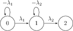
We can use these three probabilities to calculate the total mass of the sample at time $t$ by calculating the expected mass and multiplying it by the number of atoms that are present in the sample, which will not change. Only the types of atoms that are present will change: \[ \begin{aligned} \mathbb{E}[M(t)] = & N( 220 P_{00}(t) + 216 P_{01}(t) + 212 P_{02}(t) ) \\ = & N \left[ 220 e^{-\lambda_1 t} + 216 \frac{\lambda_1}{\lambda_2 - \lambda_1} \left( e^{-\lambda_1 t} - e^{-\lambda_2 t} \right) + 212\left( 1 - e^{-\lambda_1 t} - \frac{\lambda_1}{\lambda_2 - \lambda_1} \left( e^{-\lambda_1 t} - e^{-\lambda_2 t} \right) \right) \right] \\ =& N\left[ 212 + 8e^{-\lambda_1 t} + 4 \frac{\lambda_1}{\lambda_2 - \lambda_1} \left( e^{-\lambda_1 t} - e^{-\lambda_2 t} \right) \right] \end{aligned} \]

Markov chains in continuous times : Exercises

Introduction

Example problems

Problem 1

Problem 2

Problem 3

Contact Details